Artificial neural networks

The world of artificial intelligence has evolved a lot during the last decade. This advance is mainly due to the evolution of a type of algorithm called a neural network.
What are neural networks?
The theory of neural networks has existed for many years, since around the 1960s. However, we did not have the necessary mathematical tools to be able to apply them practically in our world until a few years ago.
The objective of this type of networks, known in English as neural networks , is trying to simulate the functioning of our brain to create a model that is capable of acting as an intelligence. Therefore, we can say that:
An artificial neural network is a mathematical model made up of various operations that aims to emulate the behavior of our neurons in order to learn from experience, that is, from initial data.
In short, what neural networks or artificial intelligence do is imitate human learning. Everything we know is thanks to the experience of our years of life. When we are born, our brain is blank and as we experience, it fills with knowledge and wisdom.
Neural networks work in a similar way. When initialized, they are blank and have no valuable information inside. However, as we feed the data network, it learns and is able to make decisions itself based on experience, that is, from the data we have given it.
The perceptron: the basic unit of the network
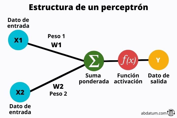
We can consider the perceptron as the basic unit of a neural network . Mathematically it is a linear binary classifier that can learn to classify two different classes.
For example, if we have a group of images of cats and dogs mixed together, a perceptron would be able to differentiate an image of a cat from one of a dog.
However, it is a very simple model that is currently only used to explain how neural networks work, which are simply many perceptrons linked together.
Let's see what parts a perceptron has:
Input values
These values are the information that enters the perceptron . These are characteristics of each of the classes to be classified.
For example, if we are talking about animals, some of the characteristics could be hair color, eye color, number of legs, hair type, etc.
These values will be transformed through a set of mathematical operations.
Ticket weights
The weights are random values that are multiplied with the input values . These weights are broadly what allows a neural network to learn. At first they are random values, but little by little, as the neural network is input, these are optimized to give the best possible results.
Activation functions
Once the characteristics have been multiplied by the weights, they are added and the resulting value is passed through what is known as the activation function.
Later we will go into detail about what this function is, but in summary, its mission is control perceptron learning or more generally of the neural network.
Thanks to these functions, neural networks are highly flexible and can learn all types of tasks.
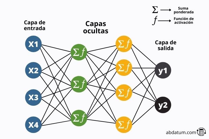
Neural network layers
We have seen, in general terms, that it is a perceptron. We can now start with artificial neural networks.
The neural networks They are simply a combination of many perceptrons. From now on, we will call these perceptrons neurons.
Therefore, an artificial neural network is simply a set of neurons joined together forming different layers .
In the following diagram we can see the typical structure of these mathematical models.
The information flows through the network until it reaches the end of the network where the results are compared with the real information. Let's look at it in more detail:
Training neural networks
What neural networks do is transform input values into output values thanks to multiple mathematical operations that they contain inside, such as addition or multiplication.
The output values have to be compared with the actual values. For example, if the neural network tells us that the image is a dog then we have to tell it if it was correct or if it was wrong.
This is achieved thanks to the loss or cost function (in English loss function ). This mathematical function tells the network how much or how little it has made a mistake.
In this way, the algorithm can optimize the weights to minimize the error function. This minimization will allow the results to be much better next time.
This is done iteratively during different cycles. These cycles are called epochs and the set of operations that are carried out to minimize the cost function is called training.
Therefore, training a neural network consists of the following:
- The weights are initialized randomly throughout the network.
- The input data are operated on the network by multiplying with the random weights and transformed by the activation functions.
- The transformed data reaches the end of the network and is compared with the real results.
- A cost function is created that determines the degree of error in the network.
- Weights are adjusted to minimize error.
- The data re-enters the network with the optimized weights and this cycle is repeated for several epochs until the error is minimal.
Backpropagation
The backpropagation algorithm was the hero of artificial intelligence. Before its discovery there was no way to train artificial neural networks.
As we mentioned before, the theory has been known for decades. However, due to the lack of computational resources and this algorithm, the networks could not be trained.
This algorithm allows us to minimize all the weights of the networks, which can be millions and millions, in a reasonable time by applying different mathematical methods of functional analysis.
The chain rule of mathematical differentiation of functions is used to find the values that make the error minimum.
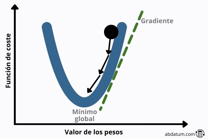
Cost function minimizers
There are multiple algorithms that allow you to optimize mathematical functions. The best known in the world of artificial intelligence is gradient descent.
This method consists of finding the vector that defines the steepest descent to reach a local minimum of the function sooner.
If the form of the loss function is quadratic, this local minimum is the global minimum, which avoids many of the problems that we will see below.
Gradient fade problem
In networks with many layers, the gradient has to propagate through all the weights of the neural network. Little by little this gradient becomes smaller and smaller.
At values very close to zero, the gradient no longer serves to optimize the neural network and, therefore, training stops.
One of the best solutions is to use what is known as skip connections . This architecture allows creating connections between distant neurons that do not come from the previous layer.
In this way, information can flow by skipping some neurons, avoiding the problem of gradient fading.
Problem of exploding gradient or explosive gradient
The explosive gradient problem is the opposite of what we have seen in the previous section. Some types of activation functions generate large numerical values.
This can lead to very high gradient values, destabilizing the neural network and generating very inaccurate predictions.
One of the methods to avoid the explosive gradient is known as gradient clipping and consists of rescaling the gradient so that the norm of the vector is within a certain range.
Types of neural networks
There are many different architectures of neural networks. Depending on how we connect them and the type of operations carried out inside them, they will correspond to one type or another.
Feedforward Neural Networks
Pre-fed neural networks or in English feed forward neural networks They constitute a type of architecture where information only flows forward, there are no loops or connections between neurons of the same layer.
They are formed by the union of different perceptrons that are responsible for transforming the input data.
This type of neural networks are the simplest and were the first to be implemented to carry out artificial intelligence tasks.
Convolutional neural networks
Convolutional networks, also known as convolutional neural networks (CNN), have an optimal architecture for working with images.
The weights of this type of network form filters that are capable of detecting different characteristics of a photo, such as shadows, edges or the shape of a human eye.
A large number of filters are applied as information flows from layer to layer. These filters are responsible for classifying the image at the end of the process.
In 2012, a model called ImageNet trained with this type of neural networks was able to classify up to 1,000 different objects in a set of one million images.
At that time, the potential of CNNs to carry out artificial intelligence with images of all types was seen.
Recurrent neural networks
Recurrent neural networks are a type of network that can form cycles, that is, a neuron can be connected to itself.
Thanks to the use of recurrence, recurrent networks such as LSTM ( Long-Short Term Memory ) or the GRUs ( Gated Recurrent Unit ) are capable of memory and remember sequences that they have previously analyzed.
This allows these artificial networks to be very effective at analyzing data that has a sequential structure. An example is the texts.
A phrase can refer to a previous event, which happened a few lines of text ago. Thanks to recurrence, these networks are able to remember and relate distant text sequences to each other.
Another type of recurrent network application is time series analysis. Many companies use this architecture to make product sales predictions based on a sequence of sales from the previous year.