ROC curves

When we use statistical models and more specifically machine learning techniques, one of the key points to interpret the results correctly is to choose the appropriate metric to measure the model error.

In classification models, one of the most used metrics to check reliability is the ROC (Receiver Operating Characteristic) curve.

This error metric measures the model's ability to correctly classify positives at different thresholds.

When we train a binary classification model we want to know if an instance is positive or negative. Let's take an example:

Imagine that we want to train a machine learning model that is capable of classifying whether an email has a virus or not. What we will obtain as a result is the probability that an email has a virus.

Normally, if the probability is above 0.5 we classify it as positive (it has a virus) and if it is below we classify it as negative (it does not have a virus).

However, if we wanted to increase the percentage of emails classified as having a virus that actually have a virus, we could raise the threshold. In this way we ensure that if we say that the email is malicious then it is very likely that it is.

However, there would be others that would have computer viruses that we would not be catching. By raising the threshold we improve what is known as model accuracy.

On the other hand, if we lower the threshold, we would improve the percentage of emails classified as malicious that they really are. In this case we would be increasing the model recall.

The ROC measure indicates the ratio of true positives versus the ratio of false positives at different classification thresholds.

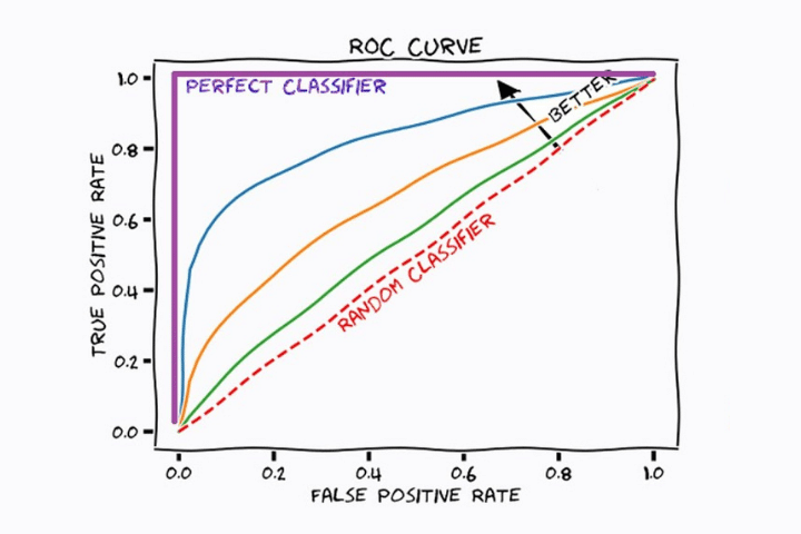
In the following image we see a graph with different curves. Each of them corresponds to a different classification machine learning model. The red straight line indicates the result of a model that classifies the samples randomly.

In all the curves we see that as the ratio of true positives (recall) increases, the number of false positives increases. This is because the threshold is decreasing and therefore most positives will be classified as positive, but some negatives will also be classified as positive.

The optimal model will be the one that increases the value of the coordinate axis (TPR) the fastest while maintaining a low value on the x-axis (FPR). In this case, the statistical model corresponding to the color blue (without taking into account the color purple, which would be the ideal) is the most appropriate.

We have seen in previous sections that the shape of the curve tells us which is the best classification model. However, visually it can be a bit complicated. For this reason, it is best to find a numerical value that quantitatively tells us which of the trained classification models best adapts to our problem.

Here comes the AUC or area under the curve. This is a simple integral calculation of the surface area under the model curve. A perfect model would have an AUC of 1 and a poor model would have a value of 0.

This metric allows us to compare different models and opt for the one that best classifies our sample.

The use of ROC and AUC is known as the ROC-AUC method.

Let's look at some examples:

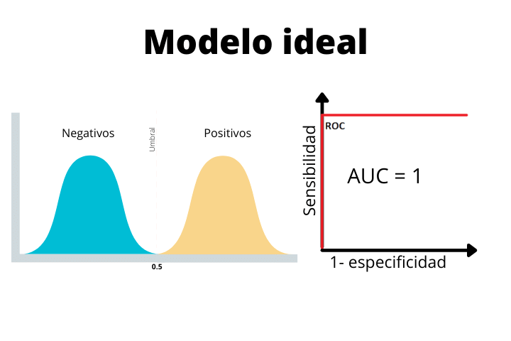
In the first image we see the case of an ideal model with a step-shaped curve and an area under the curve (AUC) of 1. This is a perfect case and we will never obtain it as a final result with real data. If you obtain such a curve in a real problem, it is highly advisable to be suspicious since such a perfect model is not common.

We see how in the ideal model, the two distributions are perfectly separated by the threshold. Since there is no overlap, the model will be able to classify the samples perfectly.

In the second case we see a real model with an AUC of 0.8. This type of curve is what we expect in a typical real-world classification problem. As we see, the two distributions overlap a bit. This will cause us to have some false positives and some false negatives.

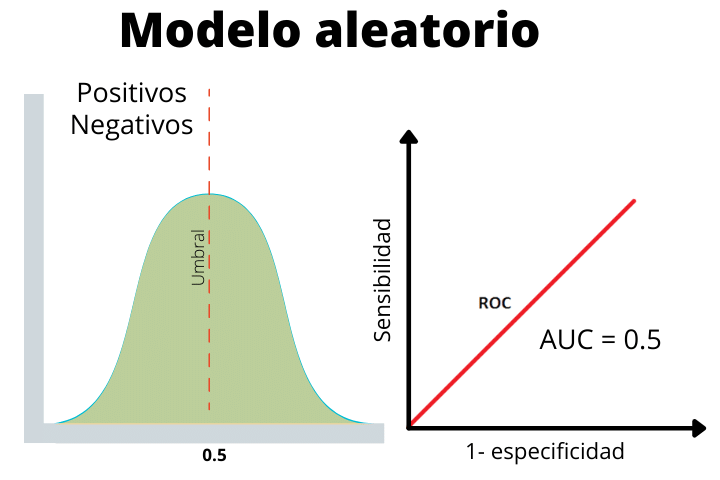
Finally we have the case of a random model where the positive and negative labels have been given at random. This line helps us determine if the performance of our model is higher than expected randomly or lower.

As we see, the two distributions overlap, therefore, it is not able to discern between a positive or a negative.